Cleaning messy data in Excel: the six functions that do it
Every useful spreadsheet starts with an ugly one. You export a customer list, a transaction dump, a payroll file — and it arrives with names typed three different ways, a whole address crammed into one cell, trailing spaces you can't even see, and dollar amounts that Excel insists are text. Before you can total it, chart it, or look anything up in it, you have to normalize it: make the values consistent so identical things actually read as identical.
It sounds like drudgery, and done by hand it is. But normalizing data is really just five or six recurring problems, and Excel has a function for each — most of them a single formula you fill down a column. Here are the six a finance operator reaches for most, in the order you usually need them.
1. Strip the invisible junk first — TRIM and CLEAN
Start here, always, because the most damaging mess is the kind you can't see. A value pasted out of a PDF, an email, or a web page almost always carries leading spaces, trailing spaces, or double spaces between words. They're invisible on screen and catastrophic underneath: "Acme " and "Acme" are different customers to Excel, so a lookup misses, a unique list shows the same name twice, and a SUMIFS quietly under-totals.
TRIM fixes it in one move: it removes spaces from the ends and collapses any run of spaces between words down to a single one. Its partner CLEAN strips non-printing characters — the stray line breaks and control codes that ride along with a paste — so =TRIM(CLEAN(A2)) is the belt-and-suspenders cleanup for anything you didn't type yourself.
=TRIM(A2)| A | B | |
|---|---|---|
| 1 | Raw | Cleaned |
| 2 | Acme Co | Acme Co |
| 3 | Length | 11 → 7 |
=TRIM(SUBSTITUTE(A2, CHAR(160), " ")) — which is a nice segue to function number five.2. Make the casing consistent — PROPER, UPPER, LOWER
A name column filled in by ten different people is a mess of jane doe, JANE DOE, and Jane DOE. None of it is wrong, exactly, but it looks unintentional and it groups badly. PROPER capitalizes the first letter of every word and lower-cases the rest, so the whole column reads as one clean Jane Doe. Its siblings UPPER and LOWER force everything to one case — UPPER for state or currency codes, LOWER for emails so they match no matter how they were typed.
PROPER isn't clever about names — it'll render McDonald as Mcdonald and LLC as Llc — so eyeball the proper nouns and acronyms after, and patch the exceptions with SUBSTITUTE. It's a normalizer, not a proofreader.
3. Split one crammed cell into many — TEXTSPLIT
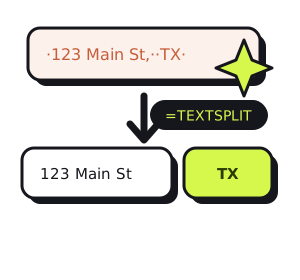
The classic import problem: a whole address — 123 Main St, Austin, TX — sitting in a single cell, when you need street, city, and state in three columns you can filter and group by. The old fix was the Text-to-Columns wizard, which you had to re-run by hand every time the data changed.
TEXTSPLIT does it as a live formula instead. Give it the delimiter — here the comma-space — and it breaks the string into pieces that spill across the columns to the right, and re-splits itself the moment the source cell changes. One delimiter splits into columns; a second, optional one starts new rows, so you can unpack a whole pasted block at once.
=TEXTSPLIT(A2, ", ")| A | B | C | D | |
|---|---|---|---|---|
| 1 | Address | Street | City | State |
| 2 | 123 Main St, Austin, TX | 123 Main St | Austin | TX |
Free · no account · no card
Get your 2027 budget built from your QuickBooks — P&L, balance sheet and cash flow, in Excel.
4. Pull out just the piece you need — TEXTBEFORE and TEXTAFTER
Sometimes you don't want to split everything — you want one specific part. The first name off a First Last column. The domain of an email. The account code before a dash. That's the job of the matched pair TEXTBEFORE and TEXTAFTER: name a marker and they hand back everything on one side of it.
=TEXTBEFORE(A2, " ")→ the first name (everything before the first space).=TEXTAFTER(A2, " ")→ the last name (everything after it). UseTEXTAFTER(A2, " ", -1)to start after the last space, so it survives middle names.=TEXTAFTER(A2, "@")→ the email domain, for grouping personal addresses apart from company ones.
They replace the old LEFT(A2, FIND(" ", A2) - 1) contortion that everyone had to look up every time — and they take a built-in fallback for when the marker isn't there, so a stray one-word entry returns your default instead of a #N/A that spreads down the column.
5. Standardize values and strip symbols — SUBSTITUTE
The last recurring mess is inconsistent values: St in one row and Street in the next, or amounts pasted as text — $1,234 — that won't add up because the $ and the comma make Excel treat them as words. SUBSTITUTE is find-and-replace you can run inside a formula, without touching the source data: it swaps every occurrence of one piece of text for another.
Use =SUBSTITUTE(A2, "St", "Street") to standardize abbreviations, and nest it to strip characters: =VALUE(SUBSTITUTE(SUBSTITUTE(A2, "$", ""), ",", "")) peels off the dollar sign and the comma, then VALUE turns the leftover text into a real number you can finally total. (One warning: SUBSTITUTE matches text anywhere, so a bare "St" also hits the St inside "Street" — include the surrounding spaces, or target a single occurrence, when that's a risk.)
6. Then it all lines up
The reason to bother with any of this shows up the moment you're done. Once a key column is trimmed, cased, and standardized, everything downstream that depends on values matching suddenly works: XLOOKUP finds its match, SUMIFS totals the right rows, and UNIQUE returns a genuinely distinct list instead of near-duplicates. Ninety percent of "the lookup is broken" is really "the data wasn't normalized first."
A practical way to work: do the cleanup in helper columns with these formulas, check it looks right, then copy and Paste Values over the original so the cleaned text is real, not formula output that breaks if you delete the source. It's the same discipline behind every tidy model — and it's the unglamorous first step of the afternoon in the case of the missing cash, where clean data was what let the real analysis begin.
Need your financials for a lender, a buyer or your accountant? Get the free financials pack →
See what an AI CFO says about your own numbers.
$99/mo, everything included. Free for 14 days, no card.